Plots and tables with reskit

2026-09-08

The aims of this vignette are to:

• illustrate usage patterns of some of the functions in {reskit}
• provide a set of test/example outputs of tables and charts derived from NHP demand model results data.

The latter may be visually compared to / validated against visualisations currently produced by the NHP Outputs app.

Firstly we load the functions in the {reskit} package.

Code

# library(reskit)
purrr::walk(dir(here::here("R"), full.names = TRUE), source)
seed <- 1871

Then we create a fake results object which consists of synthetic data created by some internal reskit functions. It ought to go without saying that the numbers in these synthetic tables are entirely fictitious and unrealistic. They exist purely to provide a test basis for the data processing and visualisation functions in this package.

This is so we don’t have to go and read in actual data for the sake of this vignette.

In real life however you would do something a bit like the steps in the next little section…

Example using azkit and reskit to download results

Here is an example of some code that you might use to access results data from Azure storage. (We’re not running it here, it’s just provided as an example.)

token <- azkit::get_auth_token()
results_container <- azkit::get_container(
  Sys.getenv("AZ_RESULTS_CONTAINER"),
  token = token
)

# use various filters to get the right dataset (PartitionKey), model version and
# scenario from a runs lookup table
results_path <- azkit::read_azure_table(
  Sys.getenv("AZ_RUNS_TABLE"),
  token = token,
  filter = "PartitionKey eq 'national' and app_version eq 'v5.1'",
  select = "aggregated_results_path"
) |>
  dplyr::pull("aggregated_results_path") |>
  grepv(pattern = "NDG2\\-zero") |>
  dplyr::first() # ensure we only get 1 path!

results <- read_results_parquet_files(results_container, results_path)

Back to our synthetic results data

OK so back in vignette world (worst theme park ever), let’s use reskit’s experimental create_demo* functions to create some fake results data.

Code

default_tbl <- create_demo_default_tbl(seed)
tretspef_losgroup_tbl <- create_demo_tretspef_losgroup_tbl(seed)
sex_agegroup_tbl <- create_demo_sex_agegroup_tbl(seed)
sex_tretspef_tbl <- create_demo_sex_tretspef_tbl(seed)
stepcounts_tbl <- create_demo_stepcounts_tbl(seed)

# fmt: skip
tbl_names <- c(
  "default", "tretspef+los_group", "sex+age_group",
  "sex+tretspef_grouped", "step_counts"
)

results <- list(
  default_tbl,
  tretspef_losgroup_tbl,
  sex_agegroup_tbl,
  sex_tretspef_tbl,
  stepcounts_tbl
) |>
  rlang::set_names(tbl_names)

We now have a real results object (an R list) to work with for the remainder of the vignette.

Moving on to the outputs (tables and charts)

Having shown one way of accessing the results parquet files, this vignette now runs through the suggested pipelines of functions that generate the NHP Outputs app tables and charts, which usually comprise in their simplest form:

• a data preparation function which creates a data frame ready to be used by:
• a visualisation function that creates a table or chart.

Some data preparation functions have sub-functions that may occsaionally be useful; there are also export* functions designed to create csv versions of prepared results data (in the same form as the data used by the visualisation function, but with all sites, measures, activity types etc included.)

Outputs: tables

“Main summary table” - overall change by Point of Delivery

This uses the “default” table (from default.parquet), passing it to the compile_principal_pod_data function which prepares the data for the table.

The only relevant filter here is for site selection.

Then the make_principal_pod_table function generates the table.

Code

results |>
  compile_principal_pod_data() |>
  make_principal_pod_table()

Point of Delivery	Baseline	Principal	Change	Percent Change
Inpatient Admissions
Non-Elective Admission	109,000	77,166	-31,834	-29%
Regular Day Attender Admission	109,000	86,141	-22,859	-21%
Regular Night Attender Admission	100,000	89,678	-10,322	-10%
Elective Admission	69,000	56,009	-12,991	-19%
Maternity Admission	45,000	41,994	-3,006	-7%
Inpatient Bed Days
Regular Day Attender Bed Days	105,000	109,058	4,058	4%
Elective Bed Days	99,000	99,257	257	0%
Non-Elective Bed Days	95,000	85,483	-9,517	-10%
Regular Night Attender Bed Days	79,000	74,273	-4,727	-6%
Maternity Bed Days	49,000	40,230	-8,770	-18%
Outpatient
Follow-up Outpatient Attendance	103,000	100,458	-2,542	-2%
Outpatient Procedure	68,000	51,664	-16,336	-24%
First Outpatient Attendance	66,000	63,935	-2,065	-3%
First Outpatient Tele-attendance	66,000	57,270	-8,730	-13%
Follow-up Outpatient Tele-attendance	50,000	47,624	-2,376	-5%
A&E
A&E Arrivals	897,000	729,576	-167,424	-19%

Now the same thing again but testing the site selection feature. We should get a similar style table but with smaller numbers as we have filtered down to just one site.

Code

results |>
  compile_principal_pod_data(sites = "site1") |>
  make_principal_pod_table()

Point of Delivery	Baseline	Principal	Change	Percent Change
Inpatient Admissions
Non-Elective Admission	78,000	55,220	-22,780	-29%
Regular Day Attender Admission	75,000	59,271	-15,729	-21%
Regular Night Attender Admission	66,000	59,187	-6,813	-10%
Elective Admission	39,000	31,658	-7,342	-19%
Maternity Admission	8,000	7,466	-534	-7%
Inpatient Bed Days
Elective Bed Days	82,000	82,213	213	0%
Non-Elective Bed Days	67,000	60,288	-6,712	-10%
Regular Night Attender Bed Days	67,000	62,991	-4,009	-6%
Regular Day Attender Bed Days	64,000	66,474	2,474	4%
Maternity Bed Days	33,000	27,093	-5,907	-18%
Outpatient
Follow-up Outpatient Attendance	64,000	62,421	-1,579	-2%
Outpatient Procedure	54,000	41,027	-12,973	-24%
First Outpatient Tele-attendance	41,000	35,577	-5,423	-13%
First Outpatient Attendance	27,000	26,155	-845	-3%
Follow-up Outpatient Tele-attendance	16,000	15,240	-760	-5%
A&E
A&E Arrivals	583,000	472,298	-110,702	-19%

The principal LoS table

This uses data from the “tretspef+los_group” results table.

With measure set to “beddays”:

Code

results |>
  compile_principal_los_data(measure = "beddays") |>
  make_principal_los_table()

Length of Stay	Baseline	Principal	Change	Percent Change
Regular Day Attender Bed Days
0 days	100,300	83,226	-17,074	-17%
1 day	79,300	65,754	-13,546	-17%
2 days	80,800	67,261	-13,539	-17%
3 days	90,100	75,723	-14,377	-16%
4-7 days	101,400	85,436	-15,964	-16%
8-14 days	95,900	80,534	-15,366	-16%
15-21 days	97,800	82,951	-14,849	-15%
22+ days	90,300	76,552	-13,748	-15%
Elective Bed Days
0 days	97,500	81,124	-16,376	-17%
1 day	100,400	83,780	-16,620	-17%
2 days	87,400	72,162	-15,238	-17%
3 days	78,300	66,917	-11,383	-15%
4-7 days	104,700	85,246	-19,454	-19%
8-14 days	92,300	76,541	-15,759	-17%
15-21 days	90,200	73,555	-16,645	-18%
22+ days	81,100	67,897	-13,203	-16%
Non-Elective Bed Days
0 days	94,100	78,204	-15,896	-17%
1 day	95,500	79,374	-16,126	-17%
2 days	82,200	71,609	-10,591	-13%
3 days	93,300	82,960	-10,340	-11%
4-7 days	81,500	67,480	-14,020	-17%
8-14 days	97,100	84,537	-12,563	-13%
15-21 days	91,600	77,736	-13,864	-15%
22+ days	85,300	73,484	-11,816	-14%
Maternity Bed Days
0 days	86,200	70,993	-15,207	-18%
1 day	83,200	66,968	-16,232	-20%
2 days	80,900	66,755	-14,145	-17%
3 days	81,500	68,332	-13,168	-16%
4-7 days	92,300	76,311	-15,989	-17%
8-14 days	84,600	72,475	-12,125	-14%
15-21 days	104,400	88,441	-15,959	-15%
22+ days	95,800	81,114	-14,686	-15%
Regular Night Attender Bed Days
0 days	82,500	66,331	-16,169	-20%
1 day	89,000	76,440	-12,560	-14%
2 days	89,900	74,860	-15,040	-17%
3 days	96,100	81,177	-14,923	-16%
4-7 days	88,700	76,878	-11,822	-13%
8-14 days	86,600	72,239	-14,361	-17%
15-21 days	88,900	72,293	-16,607	-19%
22+ days	80,900	69,209	-11,691	-14%

With measure set to “admissions”:

Code

results |>
  compile_principal_los_data(measure = "admissions", sites = "site2") |>
  make_principal_los_table()

Length of Stay	Baseline	Principal	Change	Percent Change
Elective Admission
0 days	22,200	18,731	-3,469	-16%
1 day	27,200	22,651	-4,549	-17%
2 days	28,800	24,063	-4,737	-16%
3 days	27,900	23,977	-3,923	-14%
4-7 days	27,900	23,658	-4,242	-15%
8-14 days	28,700	24,375	-4,325	-15%
15-21 days	30,000	25,127	-4,873	-16%
22+ days	27,600	23,685	-3,915	-14%
Non-Elective Admission
0 days	25,100	21,905	-3,195	-13%
1 day	26,200	22,915	-3,285	-13%
2 days	26,700	22,474	-4,226	-16%
3 days	26,400	22,887	-3,513	-13%
4-7 days	28,000	24,231	-3,769	-13%
8-14 days	28,400	24,125	-4,275	-15%
15-21 days	25,500	22,683	-2,817	-11%
22+ days	21,600	17,621	-3,979	-18%
Regular Day Attender Admission
0 days	22,900	19,884	-3,016	-13%
1 day	30,800	25,951	-4,849	-16%
2 days	26,900	23,071	-3,829	-14%
3 days	23,700	20,617	-3,083	-13%
4-7 days	25,100	21,269	-3,831	-15%
8-14 days	24,700	20,532	-4,168	-17%
15-21 days	26,800	23,333	-3,467	-13%
22+ days	24,000	20,301	-3,699	-15%
Regular Night Attender Admission
0 days	25,000	22,184	-2,816	-11%
1 day	27,300	23,134	-4,166	-15%
2 days	24,100	20,623	-3,477	-14%
3 days	26,700	22,092	-4,608	-17%
4-7 days	25,100	20,825	-4,275	-17%
8-14 days	28,900	24,373	-4,527	-16%
15-21 days	23,800	20,489	-3,311	-14%
22+ days	21,500	18,268	-3,232	-15%
Maternity Admission
0 days	22,600	19,400	-3,200	-14%
1 day	26,000	21,924	-4,076	-16%
2 days	25,300	21,385	-3,915	-15%
3 days	25,500	21,903	-3,597	-14%
4-7 days	25,300	21,904	-3,396	-13%
8-14 days	19,800	16,717	-3,083	-16%
15-21 days	22,200	18,954	-3,246	-15%
22+ days	22,200	18,744	-3,456	-16%

Outputs: charts

Impact of changes charts

For these we need to use carefully chosen combinations of measure, activity type, and pod.

Overall (“waterfall”) chart with baseline

As this is for admissions, “efficiencies” should not be shown on the y-axis.

Code

results |>
  compile_grouped_impact_data(
    measure = "admissions",
    activity_type = "ip",
    pods = c(
      "ip_elective_admission",
      "ip_maternity_admission",
      "ip_non-elective_admission"
    ),
    include_baseline = TRUE
  ) |>
  make_grouped_impact_plot()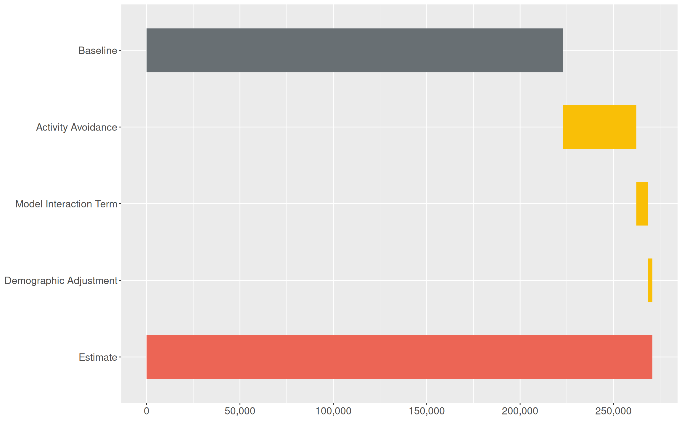

Code

results |>
  compile_grouped_impact_data(
    measure = "beddays",
    activity_type = "ip",
    pods = c(
      "ip_elective_admission",
      "ip_maternity_admission",
      "ip_non-elective_admission"
    ),
    sites = "site1",
    include_baseline = TRUE
  ) |>
  make_grouped_impact_plot()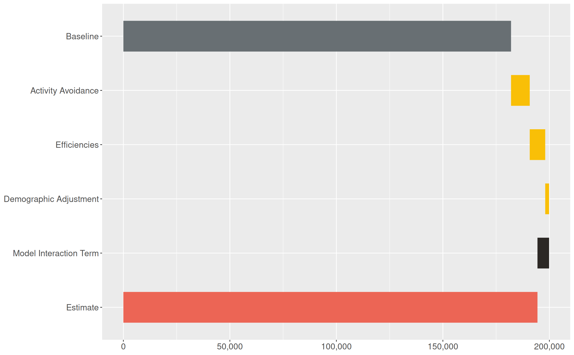

Let’s look at an outpatients chart…

Code

results |>
  compile_grouped_impact_data(
    measure = "attendances",
    activity_type = "op",
    pods = c("op_first", "op_follow-up")
  ) |>
  make_grouped_impact_plot()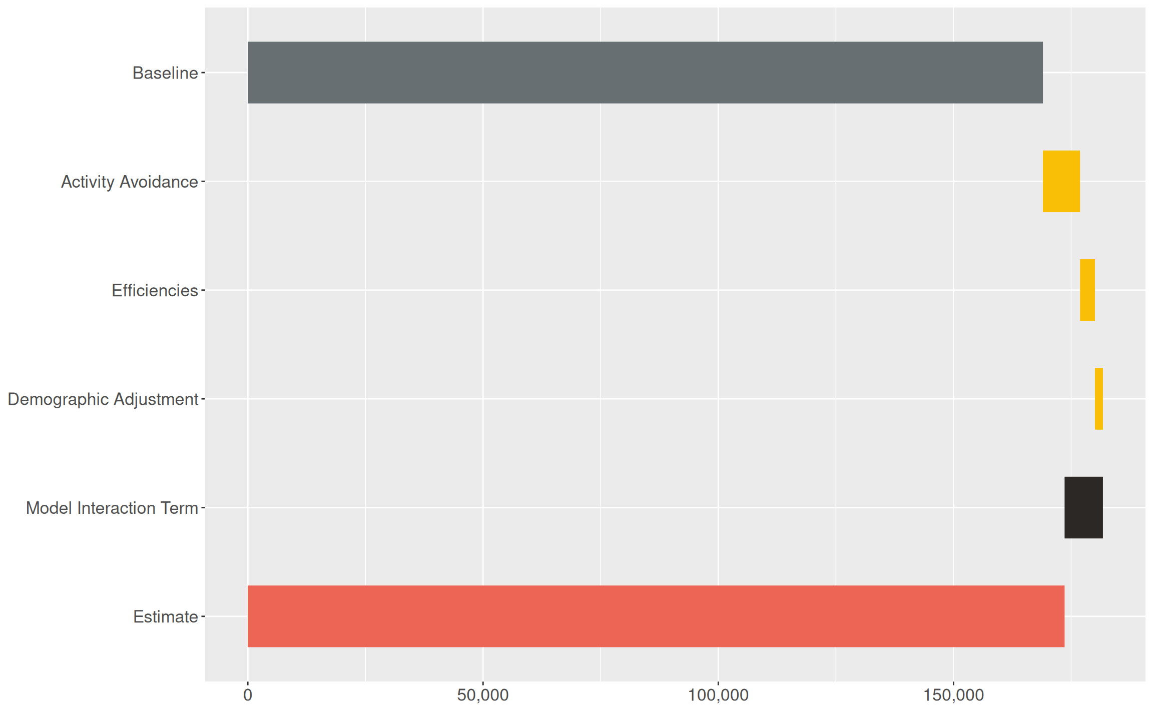

…and one without the baseline:

Code

results |>
  compile_grouped_impact_data(
    measure = "attendances",
    activity_type = "op",
    pods = c("op_first", "op_follow-up"),
    include_baseline = FALSE
  ) |>
  make_grouped_impact_plot()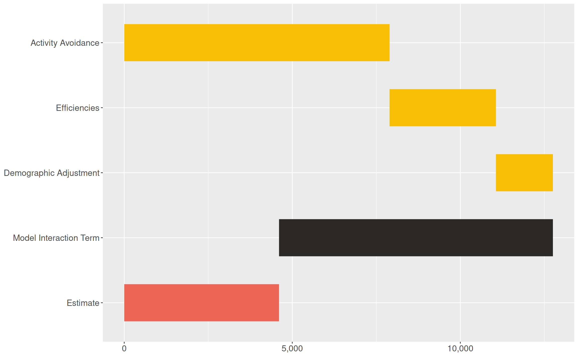

Individual change factor (TPMA) impact charts

And a couple of individual change factor charts:

Code

results |>
  compile_tpma_impact_data(
    measure = "attendances",
    activity_type = "op",
    pods = NULL
  ) |>
  make_tpma_impact_plot()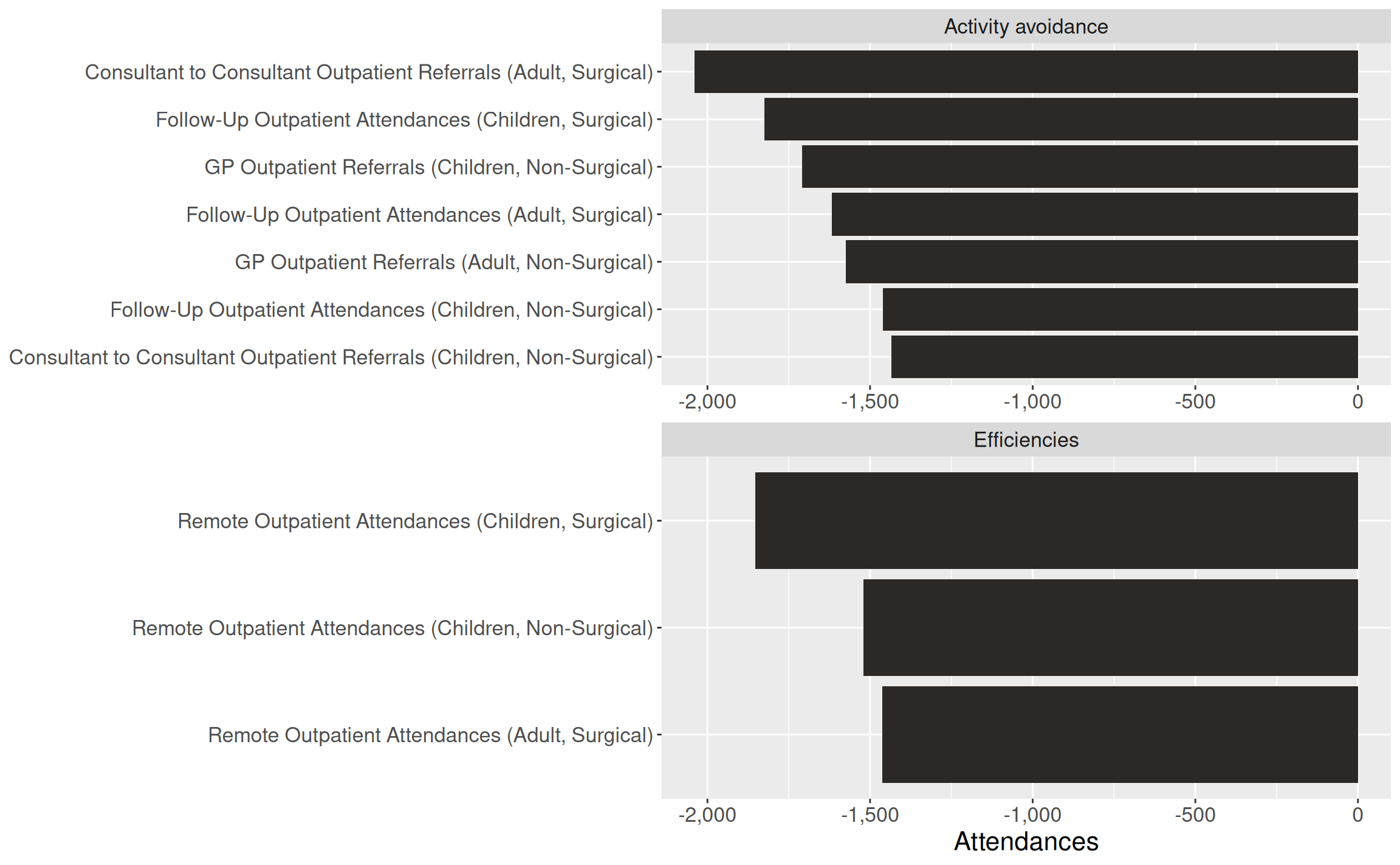

Code

results |>
  compile_tpma_impact_data(
    measure = "arrivals",
    activity_type = "aae",
    pods = NULL,
    sites = "site2"
  ) |>
  make_tpma_impact_plot()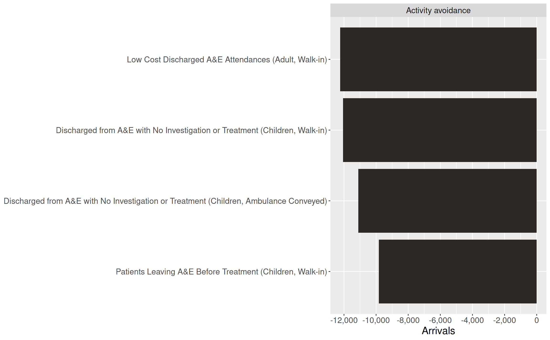

Activity in detail charts

These are even more tricky to specify as they require several arguments to be provided.

A chart by sex and age_group

Code

results |>
  compile_detailed_activity_data(
    measure = "walk-in",
    activity_type = "aae",
    aggregation = "age_group"
  ) |>
  make_detailed_activity_table(final_year = "2029/30")

Age Group	Baseline	Final (2029/30)	Change	Percent Change
Female
0	199,400	178,963	-20,437	-10%
1-4	229,500	207,405	-22,095	-10%
5-9	156,200	128,376	-27,824	-18%
10-15	142,000	123,529	-18,471	-13%
16-17	180,900	157,305	-23,595	-13%
18-34	199,200	187,863	-11,337	-6%
35-49	191,400	186,426	-4,974	-3%
50-64	188,900	160,225	-28,675	-15%
65-74	199,700	174,407	-25,293	-13%
75-84	205,100	177,127	-27,973	-14%
85+	230,100	216,937	-13,163	-6%
Male
0	220,100	180,740	-39,360	-18%
1-4	161,500	148,783	-12,717	-8%
5-9	167,100	155,750	-11,350	-7%
10-15	202,100	195,830	-6,270	-3%
16-17	209,800	177,665	-32,135	-15%
18-34	277,800	236,942	-40,858	-15%
35-49	182,200	168,698	-13,502	-7%
50-64	203,200	167,055	-36,145	-18%
65-74	254,400	228,743	-25,657	-10%
75-84	216,600	195,876	-20,724	-10%
85+	162,500	151,378	-11,122	-7%

A chart by sex and treatment speciality

Code

results |>
  compile_detailed_activity_data(
    measure = "beddays",
    activity_type = "ip",
    aggregation = "tretspef_grouped"
  ) |>
  make_detailed_activity_table(final_year = "2029/30")

Treatment Specialty	Baseline	Final (2029/30)	Change	Percent Change
Female
100: General Surgery	22,700	17,854	-4,846	-21%
101: Urology	21,700	18,076	-3,624	-17%
110: Trauma and Orthopaedic	15,200	12,041	-3,159	-21%
120: Ear Nose and Throat	23,200	18,538	-4,662	-20%
130: Ophthalmology	17,300	13,198	-4,102	-24%
140: Oral Surgery	21,300	16,352	-4,948	-23%
150: Neurosurgical	22,400	17,406	-4,994	-22%
160: Plastic Surgery	17,500	13,467	-4,033	-23%
170: Cardiothoracic Surgery	21,900	17,551	-4,349	-20%
300: General Internal Medicine	17,200	15,210	-1,990	-12%
301: Gastroenterology	13,400	10,607	-2,793	-21%
320: Cardiology	23,000	18,037	-4,963	-22%
330: Dermatology	21,400	16,440	-4,960	-23%
340: Respiratory Medicine	19,400	14,869	-4,531	-23%
400: Neurology	17,900	13,995	-3,905	-22%
410: Rheumatology	15,500	12,451	-3,049	-20%
430: Elderly Medicine	11,600	9,084	-2,516	-22%
Other	19,000	15,854	-3,146	-17%
Male
100: General Surgery	20,800	16,329	-4,471	-21%
101: Urology	15,100	12,398	-2,702	-18%
110: Trauma and Orthopaedic	22,400	18,312	-4,088	-18%
120: Ear Nose and Throat	14,900	12,064	-2,836	-19%
130: Ophthalmology	12,500	9,739	-2,761	-22%
140: Oral Surgery	13,200	9,742	-3,458	-26%
150: Neurosurgical	18,100	13,807	-4,293	-24%
160: Plastic Surgery	14,100	11,313	-2,787	-20%
170: Cardiothoracic Surgery	12,700	10,324	-2,376	-19%
300: General Internal Medicine	15,400	12,518	-2,882	-19%
301: Gastroenterology	20,500	15,665	-4,835	-24%
320: Cardiology	17,000	13,348	-3,652	-21%
330: Dermatology	21,500	16,838	-4,662	-22%
340: Respiratory Medicine	20,200	16,334	-3,866	-19%
400: Neurology	17,600	13,145	-4,455	-25%
410: Rheumatology	18,100	14,124	-3,976	-22%
430: Elderly Medicine	24,600	19,470	-5,130	-21%
Other	13,000	10,423	-2,577	-20%

Distribution tables and charts

These show the distribution across all model runs rather than just the calculated mean or principal values. For the synthetic results data we are using here, there are only 64 runs - the real model would usually use 512 or 256 runs.

Create a summary table:

Code

results |>
  compile_distribution_summary_data("median") |> # median is the default value
  make_distribution_summary_table()

Measure	Baseline	Median	Change	Percent Change	80% prediction interval
					Lower	Upper
Inpatient Non-Elective Admission
Admissions	109,000	76,488	−32,512	−30%	68,358	87,368
Bed days	95,000	84,731	−10,269	−11%	75,726	96,784
Inpatient Regular Day Attender Admission
Admissions	109,000	85,382	−23,618	−22%	76,309	97,529
Bed days	105,000	108,098	3,098	3%	96,611	123,476
Inpatient Regular Night Attender Admission
Admissions	100,000	88,888	−11,112	−11%	79,442	101,533
Bed days	79,000	73,619	−5,381	−7%	65,795	84,091
Inpatient Elective Admission
Admissions	69,000	55,516	−13,484	−20%	49,616	63,414
Bed days	99,000	98,384	−616	−1%	87,928	112,379
Inpatient Maternity Admission
Admissions	45,000	41,624	−3,376	−8%	37,201	47,545
Bed days	49,000	39,876	−9,124	−19%	35,638	45,548
Outpatient Follow-up Outpatient Attendance
Attendances	103,000	99,574	−3,426	−3%	88,993	113,739
Tele-attendances	50,000	47,205	−2,795	−6%	42,188	53,919
Outpatient Outpatient Procedure
Attendances	68,000	51,209	−16,791	−25%	45,767	58,493
Outpatient First Outpatient Attendance
Attendances	66,000	63,372	−2,628	−4%	56,637	72,388
Tele-attendances	66,000	56,766	−9,234	−14%	50,733	64,840
A&E Type 5 Department (SDEC)
Ambulance	122,000	89,518	−32,482	−27%	80,005	102,253
Walk-in	73,000	58,526	−14,474	−20%	52,307	66,852
A&E Type 2 Department
Ambulance	108,000	81,069	−26,931	−25%	72,454	92,602
Walk-in	64,000	57,064	−6,936	−11%	51,000	65,182
A&E Type 4 Department
Ambulance	94,000	68,603	−25,397	−27%	61,313	78,362
Walk-in	110,000	99,174	−10,826	−10%	88,634	113,282
A&E Type 3 Department
Ambulance	92,000	72,060	−19,940	−22%	64,402	82,311
Walk-in	83,000	85,038	2,038	2%	76,000	97,135
A&E Type 1 Department
Ambulance	88,000	68,480	−19,520	−22%	61,203	78,222
Walk-in	63,000	43,621	−19,379	−31%	38,985	49,827

An alternative:

Code

results |>
  compile_distribution_summary_data("principal") |>
  make_distribution_summary_table()

Measure	Baseline	Principal	Change	Percent Change	80% prediction interval
					Lower	Upper
Inpatient Non-Elective Admission
Admissions	109,000	77,166	−31,834	−29%	68,358	87,368
Bed days	95,000	85,483	−9,517	−10%	75,726	96,784
Inpatient Regular Day Attender Admission
Admissions	109,000	86,141	−22,859	−21%	76,309	97,529
Bed days	105,000	109,058	4,058	4%	96,611	123,476
Inpatient Regular Night Attender Admission
Admissions	100,000	89,678	−10,322	−10%	79,442	101,533
Bed days	79,000	74,273	−4,727	−6%	65,795	84,091
Inpatient Elective Admission
Admissions	69,000	56,009	−12,991	−19%	49,616	63,414
Bed days	99,000	99,257	257	0%	87,928	112,379
Inpatient Maternity Admission
Admissions	45,000	41,994	−3,006	−7%	37,201	47,545
Bed days	49,000	40,230	−8,770	−18%	35,638	45,548
Outpatient Follow-up Outpatient Attendance
Attendances	103,000	100,458	−2,542	−2%	88,993	113,739
Tele-attendances	50,000	47,624	−2,376	−5%	42,188	53,919
Outpatient Outpatient Procedure
Attendances	68,000	51,664	−16,336	−24%	45,767	58,493
Outpatient First Outpatient Attendance
Attendances	66,000	63,935	−2,065	−3%	56,637	72,388
Tele-attendances	66,000	57,270	−8,730	−13%	50,733	64,840
A&E Type 5 Department (SDEC)
Ambulance	122,000	90,313	−31,687	−26%	80,005	102,253
Walk-in	73,000	59,046	−13,954	−19%	52,307	66,852
A&E Type 2 Department
Ambulance	108,000	81,789	−26,211	−24%	72,454	92,602
Walk-in	64,000	57,571	−6,429	−10%	51,000	65,182
A&E Type 4 Department
Ambulance	94,000	69,212	−24,788	−26%	61,313	78,362
Walk-in	110,000	100,055	−9,945	−9%	88,634	113,282
A&E Type 3 Department
Ambulance	92,000	72,700	−19,300	−21%	64,402	82,311
Walk-in	83,000	85,793	2,793	3%	76,000	97,135
A&E Type 1 Department
Ambulance	88,000	69,088	−18,912	−21%	61,203	78,222
Walk-in	63,000	44,009	−18,991	−30%	38,985	49,827

Create a beeswarm chart:

Code

results |>
  compile_distribution_plot_data(measure = "walk-in", activity_type = "aae") |>
  make_beeswarm_distrib_plot()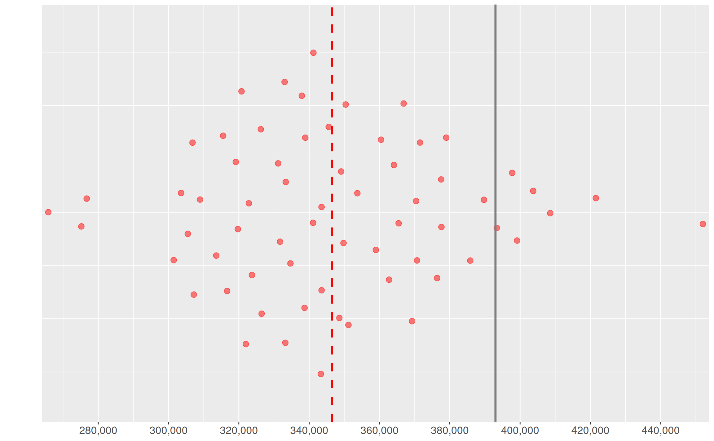

The same beeswarm chart but with the zero point shown:

Code

results |>
  compile_distribution_plot_data(measure = "walk-in", activity_type = "aae") |>
  make_beeswarm_distrib_plot(show_zero = TRUE)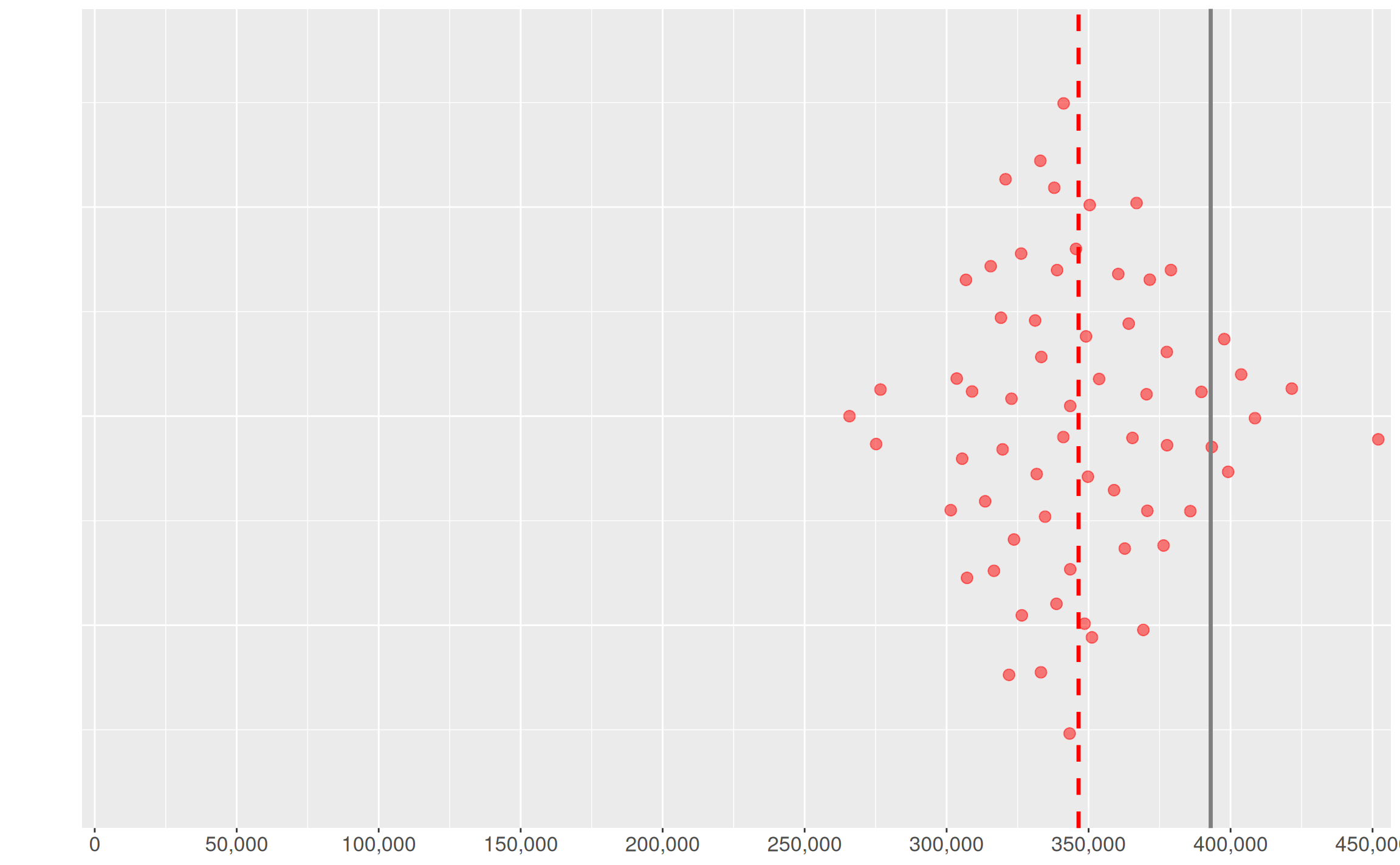

Create a cumulative distribution (ecdf) chart:

Code

results |>
  compile_distribution_plot_data(measure = "walk-in", activity_type = "aae") |>
  make_cumulative_distrib_plot()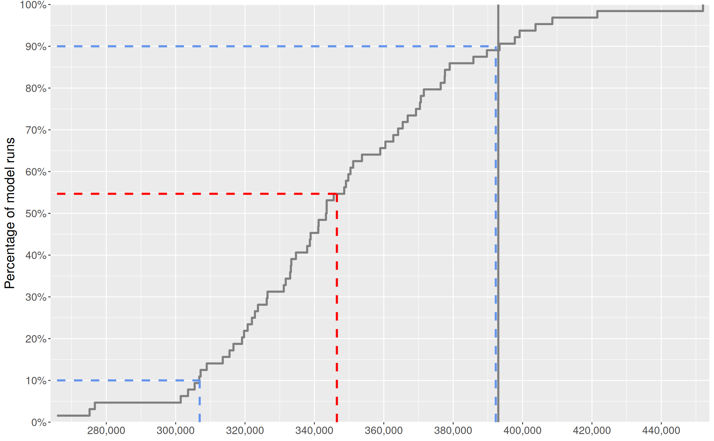

The same cumulative distribution chart but with the zero point shown:

Code

results |>
  compile_distribution_plot_data(measure = "walk-in", activity_type = "aae") |>
  make_cumulative_distrib_plot(show_zero = TRUE)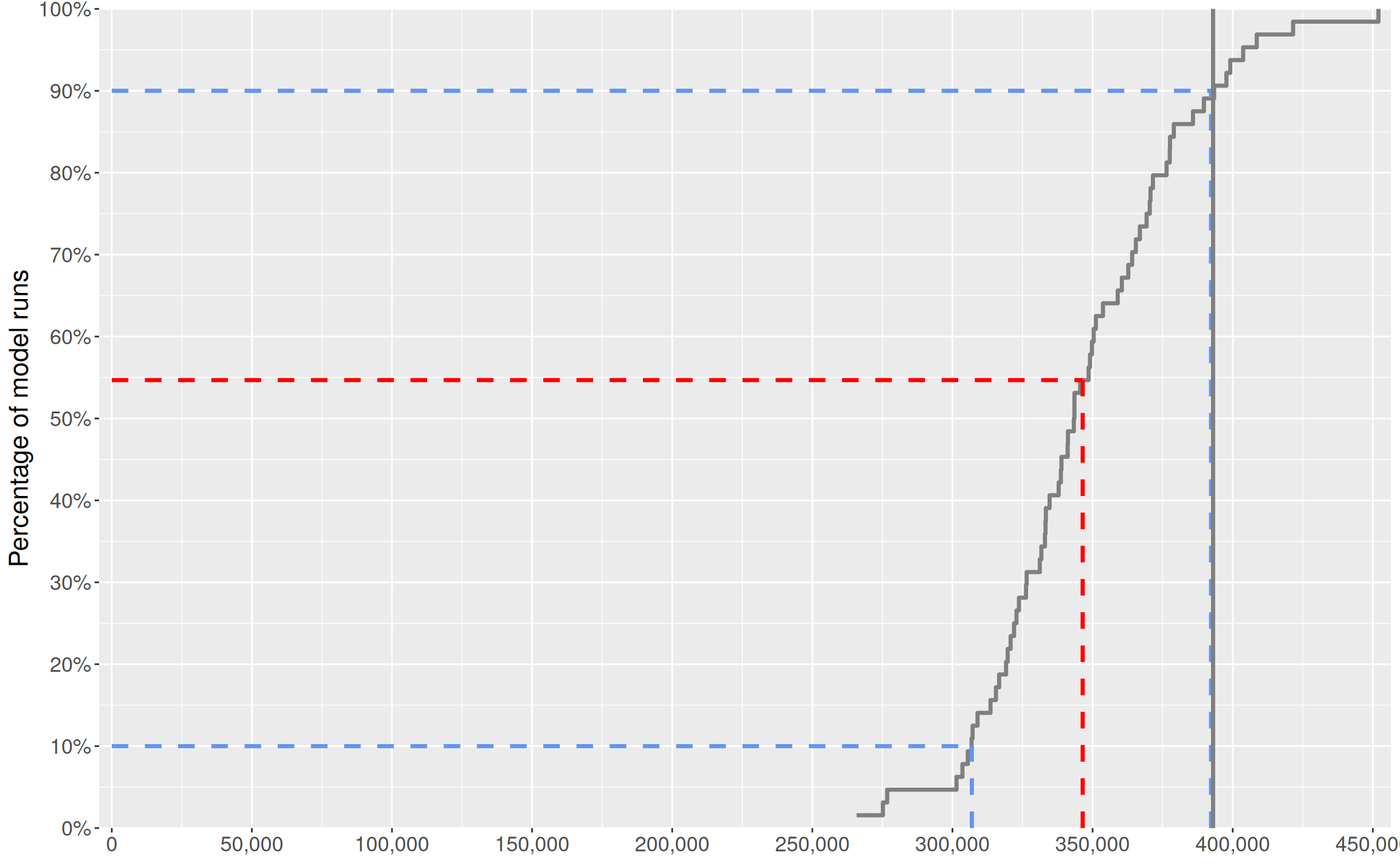

Conclusion

This vignette has included a summary of the main methods to process results data using functions from {reskit}, and to produce tables and charts.

There are many more variations on the charts shown, depending on the selection of activity type, PoD, measure and site. But this vignette shows the main processes you might need to follow - amend as necessary!