Coffee and Coding

Working with Geospatial Data in R

Aug 24, 2023

Packages we are using today

library(tidyverse)

library(sf)

library(tidygeocoder)
library(PostcodesioR)

library(osrm)

library(leaflet)

Getting boundary data

We can use the ONS’s Geoportal we can grab boundary data to generate maps

icb_url <- paste0(
  "https://services1.arcgis.com",
  "/ESMARspQHYMw9BZ9/arcgis",
  "/rest/services",
  "/Integrated_Care_Boards_April_2023_EN_BGC",
  "/FeatureServer/0/query",
  "?outFields=*&where=1%3D1&f=geojson"
)
icb_boundaries <- read_sf(icb_url)

icb_boundaries |>
  ggplot() +
  geom_sf() +
  theme_void()

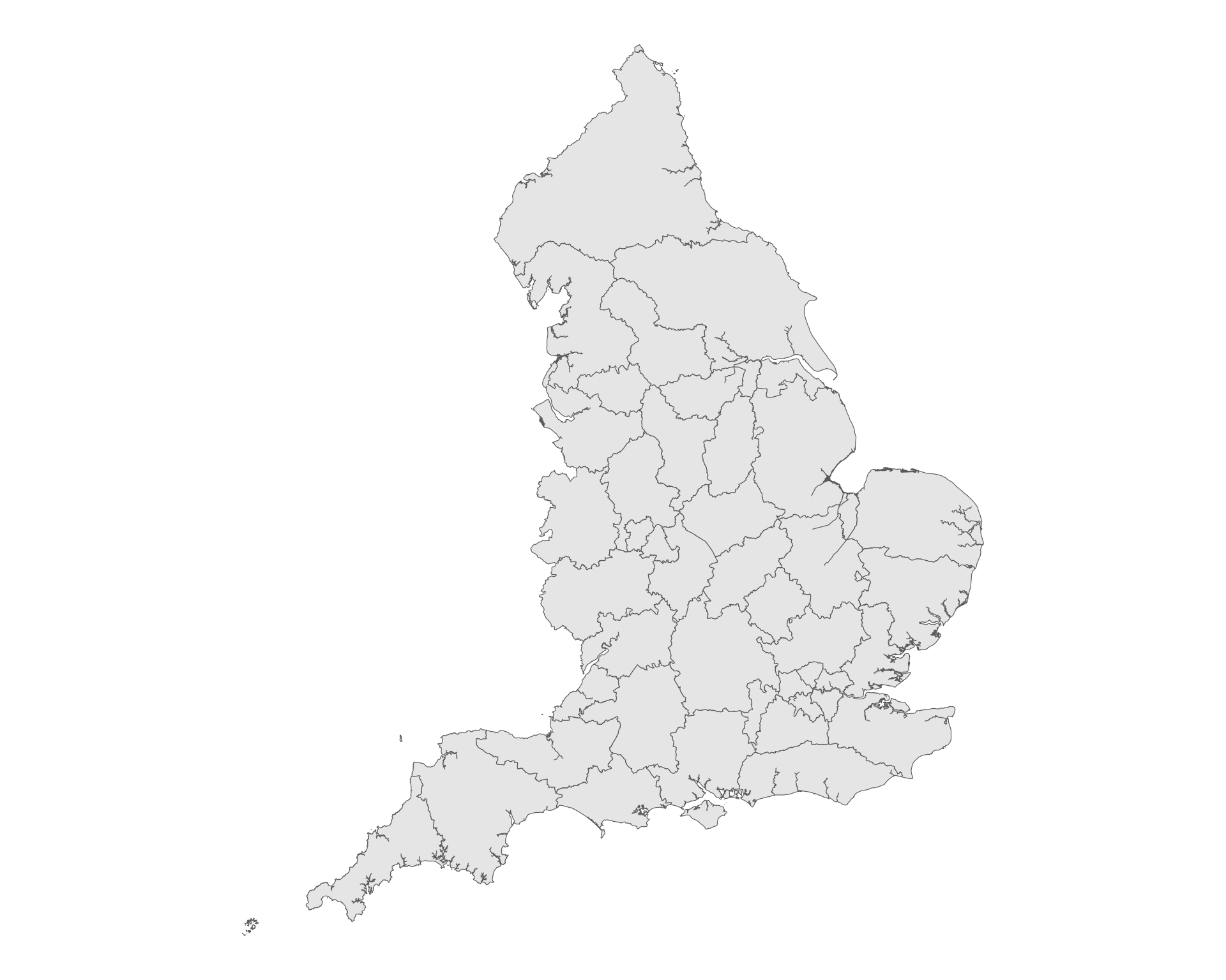
What is the `icb_boundaries` data?

icb_boundaries |>
  select(ICB23CD, ICB23NM)

Simple feature collection with 42 features and 2 fields
Geometry type: MULTIPOLYGON
Dimension:     XY
Bounding box:  xmin: -6.418667 ymin: 49.86479 xmax: 1.763706 ymax: 55.81112
Geodetic CRS:  WGS 84
# A tibble: 42 × 3
   ICB23CD   ICB23NM                                                    geometry
   <chr>     <chr>                                            <MULTIPOLYGON [°]>
 1 E54000008 NHS Cheshire and Merseyside Integrated C… (((-3.083264 53.2559, -3…
 2 E54000010 NHS Staffordshire and Stoke-on-Trent Int… (((-1.950489 53.21188, -…
 3 E54000011 NHS Shropshire, Telford and Wrekin Integ… (((-2.380794 52.99841, -…
 4 E54000013 NHS Lincolnshire Integrated Care Board    (((0.2687853 52.81584, 0…
 5 E54000015 NHS Leicester, Leicestershire and Rutlan… (((-0.7875237 52.97762, …
 6 E54000018 NHS Coventry and Warwickshire Integrated… (((-1.577608 52.67858, -…
 7 E54000019 NHS Herefordshire and Worcestershire Int… (((-2.272042 52.43972, -…
 8 E54000022 NHS Norfolk and Waveney Integrated Care … (((1.666741 52.31366, 1.…
 9 E54000023 NHS Suffolk and North East Essex Integra… (((0.8997023 51.7732, 0.…
10 E54000024 NHS Bedfordshire, Luton and Milton Keyne… (((-0.4577115 52.32009, …
# ℹ 32 more rows

Working with geospatial dataframes

We can simply join sf data frames and “regular” data frames together

icb_metrics <- icb_boundaries |>
  st_drop_geometry() |>
  select(ICB23CD) |>
  mutate(admissions = rpois(n(), 1000000))

icb_boundaries |>
  inner_join(icb_metrics, by = "ICB23CD") |>
  ggplot() +
  geom_sf(aes(fill = admissions)) +
  scale_fill_viridis_c() +
  theme_void()

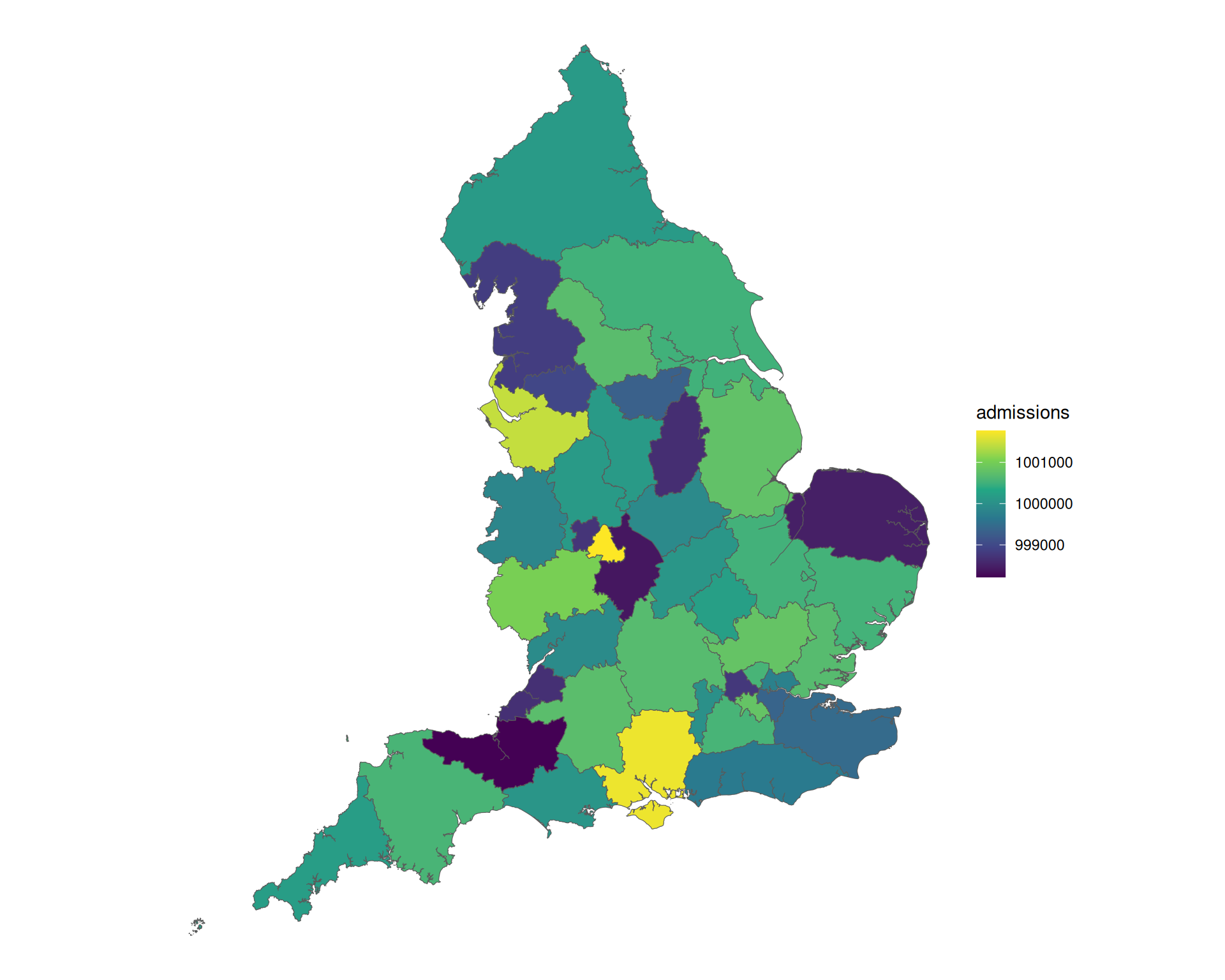
Working with geospatial data frames

We can manipulate sf objects like other data frames

london_icbs <- icb_boundaries |>
  filter(ICB23NM |> stringr::str_detect("London"))

ggplot() +
  geom_sf(data = london_icbs) +
  geom_sf(data = st_centroid(london_icbs)) +
  theme_void()

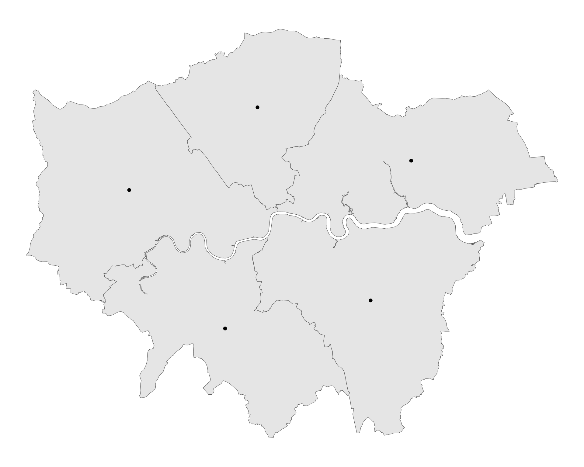
Working with geospatial data frames

Summarising the data will combine the geometries.

london_icbs |>
  summarise(area = sum(Shape__Area)) |>
  # and use geospatial functions to create calculations using the geometry
  mutate(new_area = st_area(geometry), .before = "geometry")

Simple feature collection with 1 feature and 2 fields
Geometry type: MULTIPOLYGON
Dimension:     XY
Bounding box:  xmin: -0.5102803 ymin: 51.28676 xmax: 0.3340241 ymax: 51.69188
Geodetic CRS:  WGS 84
# A tibble: 1 × 3
         area    new_area                                               geometry
*       <dbl>       [m^2]                                     <MULTIPOLYGON [°]>
1 1573336388. 1567995610. (((-0.3314819 51.43935, -0.3306676 51.43889, -0.33118…

Why the difference in area?

We are using a simplified geometry, so calculating the area will be slightly inaccurate. The original area was calculated on the non-simplified geometries.

Creating our own geospatial data

location_raw <- postcode_lookup("B2 4BJ")
glimpse(location_raw)

Rows: 1
Columns: 40
$ postcode                             <chr> "B2 4BJ"
$ quality                              <int> 1
$ eastings                             <int> 406866
$ northings                            <int> 286775
$ country                              <chr> "England"
$ nhs_ha                               <chr> "West Midlands"
$ longitude                            <dbl> -1.90033
$ latitude                             <dbl> 52.47887
$ european_electoral_region            <chr> "West Midlands"
$ primary_care_trust                   <chr> "Heart of Birmingham Teaching"
$ region                               <chr> "West Midlands"
$ lsoa                                 <chr> "Birmingham 138A"
$ msoa                                 <chr> "Birmingham 138"
$ incode                               <chr> "4BJ"
$ outcode                              <chr> "B2"
$ parliamentary_constituency           <chr> "Birmingham, Ladywood"
$ parliamentary_constituency_2024      <chr> "Birmingham Ladywood"
$ admin_district                       <chr> "Birmingham"
$ parish                               <chr> "Birmingham, unparished area"
$ admin_county                         <lgl> NA
$ date_of_introduction                 <chr> "198001"
$ admin_ward                           <chr> "Ladywood"
$ ced                                  <lgl> NA
$ ccg                                  <chr> "NHS Birmingham and Solihull"
$ nuts                                 <chr> "Birmingham"
$ pfa                                  <chr> "West Midlands"
$ admin_district_code                  <chr> "E08000025"
$ admin_county_code                    <chr> "E99999999"
$ admin_ward_code                      <chr> "E05011151"
$ parish_code                          <chr> "E43000250"
$ parliamentary_constituency_code      <chr> "E14000564"
$ parliamentary_constituency_2024_code <chr> "E14001096"
$ ccg_code                             <chr> "E38000258"
$ ccg_id_code                          <chr> "15E"
$ ced_code                             <chr> "E99999999"
$ nuts_code                            <chr> "TLG31"
$ lsoa_code                            <chr> "E01033620"
$ msoa_code                            <chr> "E02006899"
$ lau2_code                            <chr> "E08000025"
$ pfa_code                             <chr> "E23000014"

location <- location_raw |>
  st_as_sf(coords = c("eastings", "northings"), crs = 27700) |>
  select(postcode, ccg) |>
  st_transform(crs = 4326)

location

Simple feature collection with 1 feature and 2 fields
Geometry type: POINT
Dimension:     XY
Bounding box:  xmin: -1.900335 ymin: 52.47886 xmax: -1.900335 ymax: 52.47886
Geodetic CRS:  WGS 84
  postcode                         ccg                   geometry
1   B2 4BJ NHS Birmingham and Solihull POINT (-1.900335 52.47886)

Creating a geospatial data frame for all NHS Trusts

# using the NHSRtools package
# remotes::install_github("NHS-R-Community/NHSRtools")
trusts <- ods_get_trusts() |>
  filter(status == "Active") |>
  select(name, org_id, post_code) |>
  geocode(postalcode = "post_code") |>
  st_as_sf(coords = c("long", "lat"), crs = 4326)

trusts |>
  leaflet() |>
  addProviderTiles("Stamen.TonerLite") |>
  addMarkers(popup = ~name)

What are the nearest trusts to our location?

nearest_trusts <- trusts |>
  mutate(
    distance = st_distance(geometry, location)[, 1]
  ) |>
  arrange(distance) |>
  head(5)

nearest_trusts

Simple feature collection with 5 features and 4 fields
Geometry type: POINT
Dimension:     XY
Bounding box:  xmin: -1.9384 ymin: 52.4533 xmax: -1.886282 ymax: 52.48764
Geodetic CRS:  WGS 84
# A tibble: 5 × 5
  name                       org_id post_code             geometry distance
  <chr>                      <chr>  <chr>              <POINT [°]>      [m]
1 BIRMINGHAM WOMEN'S AND CH… RQ3    B4 6NH     (-1.894241 52.4849)     789.
2 BIRMINGHAM AND SOLIHULL M… RXT    B1 3RB    (-1.917663 52.48416)    1313.
3 BIRMINGHAM COMMUNITY HEAL… RYW    B7 4BN    (-1.886282 52.48754)    1356.
4 SANDWELL AND WEST BIRMING… RXK    B18 7QH   (-1.930203 52.48764)    2246.
5 UNIVERSITY HOSPITALS BIRM… RRK    B15 2GW      (-1.9384 52.4533)    3838.

Let’s find driving routes to these trusts

routes <- nearest_trusts |>
  mutate(
    route = map(geometry, ~ osrmRoute(location, st_coordinates(.x)))
  ) |>
  st_drop_geometry() |>
  rename(straight_line_distance = distance) |>
  unnest(route) |>
  st_as_sf()

routes

Simple feature collection with 5 features and 8 fields
Geometry type: LINESTRING
Dimension:     XY
Bounding box:  xmin: -1.93846 ymin: 52.45316 xmax: -1.88527 ymax: 52.49279
Geodetic CRS:  WGS 84
# A tibble: 5 × 9
  name     org_id post_code straight_line_distance src   dst   duration distance
  <chr>    <chr>  <chr>                        [m] <chr> <chr>    <dbl>    <dbl>
1 BIRMING… RQ3    B4 6NH                      789. 1     dst       5.77     3.09
2 BIRMING… RXT    B1 3RB                     1313. 1     dst       6.84     4.14
3 BIRMING… RYW    B7 4BN                     1356. 1     dst       7.59     4.29
4 SANDWEL… RXK    B18 7QH                    2246. 1     dst       8.78     4.95
5 UNIVERS… RRK    B15 2GW                    3838. 1     dst      10.6      4.67
# ℹ 1 more variable: geometry <LINESTRING [°]>

Let’s show the routes

leaflet(routes) |>
  addTiles() |>
  addMarkers(data = location) |>
  addPolylines(color = "black", weight = 3, opacity = 1) |>
  addCircleMarkers(data = nearest_trusts, radius = 4, opacity = 1, fillOpacity = 1)

We can use `{osrm}` to calculate isochrones

iso <- osrmIsochrone(location, breaks = seq(0, 60, 15), res = 10)

isochrone_ids <- unique(iso$id)

pal <- colorFactor(
  viridis::viridis(length(isochrone_ids)),
  isochrone_ids
)

leaflet(location) |>
  addProviderTiles("Stamen.TonerLite") |>
  addMarkers() |>
  addPolygons(
    data = iso,
    fillColor = ~ pal(id),
    color = "#000000",
    weight = 1
  )

What trusts are in the isochrones?

The summarise() function will “union” the geometry

summarise(iso)

Simple feature collection with 1 feature and 0 fields
Geometry type: POLYGON
Dimension:     XY
Bounding box:  xmin: -2.913575 ymin: 51.98062 xmax: -0.8502164 ymax: 53.1084
Geodetic CRS:  WGS 84
                        geometry
1 POLYGON ((-1.541014 52.9693...

What trusts are in the isochrones?

We can use this with a geo-filter to find the trusts in the isochrone

# also works
trusts_in_iso <- trusts |>
  st_filter(
    summarise(iso),
    .predicate = st_within
  )

trusts_in_iso

Simple feature collection with 31 features and 3 fields
Geometry type: POINT
Dimension:     XY
Bounding box:  xmin: -2.793386 ymin: 52.19205 xmax: -1.10302 ymax: 53.01015
Geodetic CRS:  WGS 84
# A tibble: 31 × 4
   name                               org_id post_code             geometry
 * <chr>                              <chr>  <chr>              <POINT [°]>
 1 BIRMINGHAM AND SOLIHULL MENTAL HE… RXT    B1 3RB    (-1.917663 52.48416)
 2 BIRMINGHAM COMMUNITY HEALTHCARE N… RYW    B7 4BN    (-1.886282 52.48754)
 3 BIRMINGHAM WOMEN'S AND CHILDREN'S… RQ3    B4 6NH     (-1.894241 52.4849)
 4 BIRMINGHAM WOMEN'S NHS FOUNDATION… RLU    B15 2TG   (-1.942861 52.45325)
 5 BURTON HOSPITALS NHS FOUNDATION T… RJF    DE13 0RB  (-1.656667 52.81774)
 6 COVENTRY AND WARWICKSHIRE PARTNER… RYG    CV6 6NY    (-1.48692 52.45659)
 7 DERBYSHIRE HEALTHCARE NHS FOUNDAT… RXM    DE22 3LZ  (-1.512896 52.91831)
 8 DUDLEY INTEGRATED HEALTH AND CARE… RYK    DY5 1RU    (-2.11786 52.48176)
 9 GEORGE ELIOT HOSPITAL NHS TRUST    RLT    CV10 7DJ   (-1.47844 52.51258)
10 HEART OF ENGLAND NHS FOUNDATION T… RR1    B9 5ST     (-1.828759 52.4781)
# ℹ 21 more rows

What trusts are in the isochrones?

leaflet(trusts_in_iso) |>
  addProviderTiles("Stamen.TonerLite") |>
  addMarkers() |>
  addPolygons(
    data = iso,
    fillColor = ~pal(id),
    color = "#000000",
    weight = 1
  )

Doing the same but within a radius

r <- 25000

trusts_in_radius <- trusts |>
  st_filter(
    location,
    .predicate = st_is_within_distance,
    dist = r
  )

# transforming gives us a pretty smooth circle
radius <- location |>
  st_transform(crs = 27700) |>
  st_buffer(dist = r) |>
  st_transform(crs = 4326)

leaflet(trusts_in_radius) |>
  addProviderTiles("Stamen.TonerLite") |>
  addMarkers() |>
  addPolygons(
    data = radius,
    color = "#000000",
    weight = 1
  )

Coffee and Coding

Packages we are using today

Getting boundary data

What is the icb_boundaries data?

Working with geospatial dataframes

Working with geospatial data frames

Working with geospatial data frames

Creating our own geospatial data

Creating a geospatial data frame for all NHS Trusts

What are the nearest trusts to our location?

Let’s find driving routes to these trusts

Let’s show the routes

We can use {osrm} to calculate isochrones

What trusts are in the isochrones?

What trusts are in the isochrones?

What trusts are in the isochrones?

Doing the same but within a radius

Further reading

What is the `icb_boundaries` data?

We can use `{osrm}` to calculate isochrones